
Zaoqi's Blog -> Python数据分析教程 -> 图解Pandas ->
官方教程 - 10分钟入门pandas
官方教程 - 10分钟入门pandas
教程译自10 Minutes to pandas,有删改,点击直达最新文档地址
在线刷题
检查 or 强化 Pandas 数据分析操作?👉在线体验「Pandas进阶修炼300题」
Note
本页面代码可以在线编辑、执行!
首先导入 Python 数据处理中常用的三个库,如果没有需要提前使用 pip 安装
import numpy as np
import pandas as pd
import matplotlib.pyplot as plt
注:本教程基于Pandas0.18.0版本,因版本不同可能有些代码无法成功执行,请自行查阅解决办法
创建数据
使用pd.Series创建Series对象
s = pd.Series([1,3,5,np.nan,6,8])
s
0    1.0
1    3.0
2    5.0
3    NaN
4    6.0
5    8.0
dtype: float64
通过numpy的array数据来创建DataFrame对象
dates = pd.date_range('20130101', periods=6)
dates
DatetimeIndex(['2013-01-01', '2013-01-02', '2013-01-03', '2013-01-04',
               '2013-01-05', '2013-01-06'],
              dtype='datetime64[ns]', freq='D')
df = pd.DataFrame(np.random.randn(6,4), index=dates, columns=list('ABCD'))
df
| A | B | C | D | |
|---|---|---|---|---|
| 2013-01-01 | 0.342275 | -0.333060 | -0.294502 | 1.808311 |
| 2013-01-02 | -0.010251 | -0.322083 | -0.992557 | -0.960891 |
| 2013-01-03 | -0.344072 | -1.185725 | 0.674009 | -0.716058 |
| 2013-01-04 | -0.235446 | -1.721794 | -1.265767 | 0.242253 |
| 2013-01-05 | 3.074955 | 1.848873 | 1.813445 | -0.795627 |
| 2013-01-06 | -0.039975 | 1.090794 | -0.605099 | -1.111459 |
通过字典创建DataFrame对象
df2 = pd.DataFrame({ 'A' : 1.,
                     'B' : pd.Timestamp('20130102'),
                     'C' : pd.Series(1,index=list(range(4)),dtype='float32'),
                     'D' : np.array([3] * 4,dtype='int32'),
                     'E' : pd.Categorical(["test","train","test","train"]),
                     'F' : 'foo' })
df2
| A | B | C | D | E | F | |
|---|---|---|---|---|---|---|
| 0 | 1.0 | 2013-01-02 | 1.0 | 3 | test | foo |
| 1 | 1.0 | 2013-01-02 | 1.0 | 3 | train | foo |
| 2 | 1.0 | 2013-01-02 | 1.0 | 3 | test | foo |
| 3 | 1.0 | 2013-01-02 | 1.0 | 3 | train | foo |
df2.dtypes
A           float64
B    datetime64[ns]
C           float32
D             int32
E          category
F            object
dtype: object
dir(df2)
['A',
 'B',
 'C',
 'D',
 'E',
 'F',
 'T',
 '_AXIS_LEN',
 '_AXIS_NAMES',
 '_AXIS_NUMBERS',
 '_AXIS_ORDERS',
 '_AXIS_REVERSED',
 '_AXIS_TO_AXIS_NUMBER',
 '__abs__',
 '__add__',
 '__and__',
 '__annotations__',
 '__array__',
 '__array_priority__',
 '__array_wrap__',
 '__bool__',
 '__class__',
 '__contains__',
 '__copy__',
 '__deepcopy__',
 '__delattr__',
 '__delitem__',
 '__dict__',
 '__dir__',
 '__div__',
 '__doc__',
 '__eq__',
 '__finalize__',
 '__floordiv__',
 '__format__',
 '__ge__',
 '__getattr__',
 '__getattribute__',
 '__getitem__',
 '__getstate__',
 '__gt__',
 '__hash__',
 '__iadd__',
 '__iand__',
 '__ifloordiv__',
 '__imod__',
 '__imul__',
 '__init__',
 '__init_subclass__',
 '__invert__',
 '__ior__',
 '__ipow__',
 '__isub__',
 '__iter__',
 '__itruediv__',
 '__ixor__',
 '__le__',
 '__len__',
 '__lt__',
 '__matmul__',
 '__mod__',
 '__module__',
 '__mul__',
 '__ne__',
 '__neg__',
 '__new__',
 '__nonzero__',
 '__or__',
 '__pos__',
 '__pow__',
 '__radd__',
 '__rand__',
 '__rdiv__',
 '__reduce__',
 '__reduce_ex__',
 '__repr__',
 '__rfloordiv__',
 '__rmatmul__',
 '__rmod__',
 '__rmul__',
 '__ror__',
 '__round__',
 '__rpow__',
 '__rsub__',
 '__rtruediv__',
 '__rxor__',
 '__setattr__',
 '__setitem__',
 '__setstate__',
 '__sizeof__',
 '__str__',
 '__sub__',
 '__subclasshook__',
 '__truediv__',
 '__weakref__',
 '__xor__',
 '_accessors',
 '_add_numeric_operations',
 '_add_series_or_dataframe_operations',
 '_agg_by_level',
 '_agg_examples_doc',
 '_agg_summary_and_see_also_doc',
 '_aggregate',
 '_aggregate_multiple_funcs',
 '_align_frame',
 '_align_series',
 '_box_col_values',
 '_builtin_table',
 '_can_fast_transpose',
 '_check_inplace_setting',
 '_check_is_chained_assignment_possible',
 '_check_label_or_level_ambiguity',
 '_check_setitem_copy',
 '_clear_item_cache',
 '_clip_with_one_bound',
 '_clip_with_scalar',
 '_combine_frame',
 '_consolidate',
 '_consolidate_inplace',
 '_construct_axes_dict',
 '_construct_axes_from_arguments',
 '_construct_result',
 '_constructor',
 '_constructor_expanddim',
 '_constructor_sliced',
 '_convert',
 '_count_level',
 '_cython_table',
 '_data',
 '_deprecations',
 '_dir_additions',
 '_dir_deletions',
 '_drop_axis',
 '_drop_labels_or_levels',
 '_ensure_valid_index',
 '_find_valid_index',
 '_from_arrays',
 '_get_agg_axis',
 '_get_axis',
 '_get_axis_name',
 '_get_axis_number',
 '_get_axis_resolvers',
 '_get_block_manager_axis',
 '_get_bool_data',
 '_get_cacher',
 '_get_cleaned_column_resolvers',
 '_get_column_array',
 '_get_cython_func',
 '_get_index_resolvers',
 '_get_item_cache',
 '_get_label_or_level_values',
 '_get_numeric_data',
 '_get_value',
 '_getitem_bool_array',
 '_getitem_multilevel',
 '_gotitem',
 '_indexed_same',
 '_info_axis',
 '_info_axis_name',
 '_info_axis_number',
 '_info_repr',
 '_init_mgr',
 '_internal_names',
 '_internal_names_set',
 '_is_builtin_func',
 '_is_cached',
 '_is_copy',
 '_is_homogeneous_type',
 '_is_label_or_level_reference',
 '_is_label_reference',
 '_is_level_reference',
 '_is_mixed_type',
 '_is_view',
 '_iset_item',
 '_iter_column_arrays',
 '_ix',
 '_ixs',
 '_join_compat',
 '_maybe_cache_changed',
 '_maybe_update_cacher',
 '_metadata',
 '_needs_reindex_multi',
 '_obj_with_exclusions',
 '_protect_consolidate',
 '_reduce',
 '_reindex_axes',
 '_reindex_columns',
 '_reindex_index',
 '_reindex_multi',
 '_reindex_with_indexers',
 '_replace_columnwise',
 '_repr_data_resource_',
 '_repr_fits_horizontal_',
 '_repr_fits_vertical_',
 '_repr_html_',
 '_repr_latex_',
 '_reset_cache',
 '_reset_cacher',
 '_sanitize_column',
 '_selected_obj',
 '_selection',
 '_selection_list',
 '_selection_name',
 '_series',
 '_set_as_cached',
 '_set_axis',
 '_set_axis_name',
 '_set_is_copy',
 '_set_item',
 '_set_value',
 '_setitem_array',
 '_setitem_frame',
 '_setitem_slice',
 '_slice',
 '_stat_axis',
 '_stat_axis_name',
 '_stat_axis_number',
 '_take_with_is_copy',
 '_to_dict_of_blocks',
 '_try_aggregate_string_function',
 '_typ',
 '_update_inplace',
 '_validate_dtype',
 '_values',
 '_where',
 'abs',
 'add',
 'add_prefix',
 'add_suffix',
 'agg',
 'aggregate',
 'align',
 'all',
 'any',
 'append',
 'apply',
 'applymap',
 'asfreq',
 'asof',
 'assign',
 'astype',
 'at',
 'at_time',
 'attrs',
 'axes',
 'backfill',
 'between_time',
 'bfill',
 'bool',
 'boxplot',
 'clip',
 'columns',
 'combine',
 'combine_first',
 'compare',
 'convert_dtypes',
 'copy',
 'corr',
 'corrwith',
 'count',
 'cov',
 'cummax',
 'cummin',
 'cumprod',
 'cumsum',
 'describe',
 'diff',
 'div',
 'divide',
 'dot',
 'drop',
 'drop_duplicates',
 'droplevel',
 'dropna',
 'dtypes',
 'duplicated',
 'empty',
 'eq',
 'equals',
 'eval',
 'ewm',
 'expanding',
 'explode',
 'ffill',
 'fillna',
 'filter',
 'first',
 'first_valid_index',
 'floordiv',
 'from_dict',
 'from_records',
 'ge',
 'get',
 'groupby',
 'gt',
 'head',
 'hist',
 'iat',
 'idxmax',
 'idxmin',
 'iloc',
 'index',
 'infer_objects',
 'info',
 'insert',
 'interpolate',
 'isin',
 'isna',
 'isnull',
 'items',
 'iteritems',
 'iterrows',
 'itertuples',
 'join',
 'keys',
 'kurt',
 'kurtosis',
 'last',
 'last_valid_index',
 'le',
 'loc',
 'lookup',
 'lt',
 'mad',
 'mask',
 'max',
 'mean',
 'median',
 'melt',
 'memory_usage',
 'merge',
 'min',
 'mod',
 'mode',
 'mul',
 'multiply',
 'ndim',
 'ne',
 'nlargest',
 'notna',
 'notnull',
 'nsmallest',
 'nunique',
 'pad',
 'pct_change',
 'pipe',
 'pivot',
 'pivot_table',
 'plot',
 'pop',
 'pow',
 'prod',
 'product',
 'quantile',
 'query',
 'radd',
 'rank',
 'rdiv',
 'reindex',
 'reindex_like',
 'rename',
 'rename_axis',
 'reorder_levels',
 'replace',
 'resample',
 'reset_index',
 'rfloordiv',
 'rmod',
 'rmul',
 'rolling',
 'round',
 'rpow',
 'rsub',
 'rtruediv',
 'sample',
 'select_dtypes',
 'sem',
 'set_axis',
 'set_index',
 'shape',
 'shift',
 'size',
 'skew',
 'slice_shift',
 'sort_index',
 'sort_values',
 'squeeze',
 'stack',
 'std',
 'style',
 'sub',
 'subtract',
 'sum',
 'swapaxes',
 'swaplevel',
 'tail',
 'take',
 'to_clipboard',
 'to_csv',
 'to_dict',
 'to_excel',
 'to_feather',
 'to_gbq',
 'to_hdf',
 'to_html',
 'to_json',
 'to_latex',
 'to_markdown',
 'to_numpy',
 'to_parquet',
 'to_period',
 'to_pickle',
 'to_records',
 'to_sql',
 'to_stata',
 'to_string',
 'to_timestamp',
 'to_xarray',
 'transform',
 'transpose',
 'truediv',
 'truncate',
 'tz_convert',
 'tz_localize',
 'unstack',
 'update',
 'value_counts',
 'values',
 'var',
 'where',
 'xs']
数据查看
基本方法,务必掌握,更多相关查看数据的方法可以参与官方文档
下面分别是查看数据的顶部和尾部的方法
df.head()
| A | B | C | D | |
|---|---|---|---|---|
| 2013-01-01 | 0.342275 | -0.333060 | -0.294502 | 1.808311 |
| 2013-01-02 | -0.010251 | -0.322083 | -0.992557 | -0.960891 |
| 2013-01-03 | -0.344072 | -1.185725 | 0.674009 | -0.716058 |
| 2013-01-04 | -0.235446 | -1.721794 | -1.265767 | 0.242253 |
| 2013-01-05 | 3.074955 | 1.848873 | 1.813445 | -0.795627 |
df.tail(3)
| A | B | C | D | |
|---|---|---|---|---|
| 2013-01-04 | -0.235446 | -1.721794 | -1.265767 | 0.242253 |
| 2013-01-05 | 3.074955 | 1.848873 | 1.813445 | -0.795627 |
| 2013-01-06 | -0.039975 | 1.090794 | -0.605099 | -1.111459 |
查看DataFrame对象的索引,列名,数据信息
df.index
DatetimeIndex(['2013-01-01', '2013-01-02', '2013-01-03', '2013-01-04',
               '2013-01-05', '2013-01-06'],
              dtype='datetime64[ns]', freq='D')
df.columns
Index(['A', 'B', 'C', 'D'], dtype='object')
df.values
array([[ 0.34227537, -0.33306022, -0.29450173,  1.80831125],
       [-0.01025096, -0.3220833 , -0.99255656, -0.96089093],
       [-0.34407203, -1.18572491,  0.67400852, -0.71605802],
       [-0.2354458 , -1.7217938 , -1.26576668,  0.24225255],
       [ 3.07495472,  1.84887323,  1.81344527, -0.79562727],
       [-0.0399747 ,  1.0907938 , -0.60509926, -1.11145858]])
描述性统计
df.describe()
| A | B | C | D | |
|---|---|---|---|---|
| count | 6.000000 | 6.000000 | 6.000000 | 6.000000 |
| mean | 0.464581 | -0.103833 | -0.111745 | -0.255579 |
| std | 1.300231 | 1.351197 | 1.158288 | 1.117244 |
| min | -0.344072 | -1.721794 | -1.265767 | -1.111459 |
| 25% | -0.186578 | -0.972559 | -0.895692 | -0.919575 |
| 50% | -0.025113 | -0.327572 | -0.449800 | -0.755843 |
| 75% | 0.254144 | 0.737575 | 0.431881 | 0.002675 |
| max | 3.074955 | 1.848873 | 1.813445 | 1.808311 |
数据转置
df.T
| 2013-01-01 | 2013-01-02 | 2013-01-03 | 2013-01-04 | 2013-01-05 | 2013-01-06 | |
|---|---|---|---|---|---|---|
| A | 0.342275 | -0.010251 | -0.344072 | -0.235446 | 3.074955 | -0.039975 |
| B | -0.333060 | -0.322083 | -1.185725 | -1.721794 | 1.848873 | 1.090794 |
| C | -0.294502 | -0.992557 | 0.674009 | -1.265767 | 1.813445 | -0.605099 |
| D | 1.808311 | -0.960891 | -0.716058 | 0.242253 | -0.795627 | -1.111459 |
根据列名排序
df.sort_index(axis=1, ascending=False)
| D | C | B | A | |
|---|---|---|---|---|
| 2013-01-01 | 1.808311 | -0.294502 | -0.333060 | 0.342275 |
| 2013-01-02 | -0.960891 | -0.992557 | -0.322083 | -0.010251 |
| 2013-01-03 | -0.716058 | 0.674009 | -1.185725 | -0.344072 |
| 2013-01-04 | 0.242253 | -1.265767 | -1.721794 | -0.235446 |
| 2013-01-05 | -0.795627 | 1.813445 | 1.848873 | 3.074955 |
| 2013-01-06 | -1.111459 | -0.605099 | 1.090794 | -0.039975 |
根据B列数值排序
df.sort_values(by='B')
| A | B | C | D | |
|---|---|---|---|---|
| 2013-01-04 | -0.235446 | -1.721794 | -1.265767 | 0.242253 |
| 2013-01-03 | -0.344072 | -1.185725 | 0.674009 | -0.716058 |
| 2013-01-01 | 0.342275 | -0.333060 | -0.294502 | 1.808311 |
| 2013-01-02 | -0.010251 | -0.322083 | -0.992557 | -0.960891 |
| 2013-01-06 | -0.039975 | 1.090794 | -0.605099 | -1.111459 |
| 2013-01-05 | 3.074955 | 1.848873 | 1.813445 | -0.795627 |
数据选取
官方建议使用优化的熊猫数据访问方法.at,.iat,.loc和.iloc,部分较早的pandas版本可以使用.ix
这些选取函数的使用需要熟练掌握,我也曾写过相关文章帮助理解
使用[]选取数据
选取单列数据,等效于df.A:
df['A']
2013-01-01    0.342275
2013-01-02   -0.010251
2013-01-03   -0.344072
2013-01-04   -0.235446
2013-01-05    3.074955
2013-01-06   -0.039975
Freq: D, Name: A, dtype: float64
按行选取数据,使用[]
df[0:3]
| A | B | C | D | |
|---|---|---|---|---|
| 2013-01-01 | 0.342275 | -0.333060 | -0.294502 | 1.808311 |
| 2013-01-02 | -0.010251 | -0.322083 | -0.992557 | -0.960891 |
| 2013-01-03 | -0.344072 | -1.185725 | 0.674009 | -0.716058 |
df['20130102':'20130104']
| A | B | C | D | |
|---|---|---|---|---|
| 2013-01-02 | -0.010251 | -0.322083 | -0.992557 | -0.960891 |
| 2013-01-03 | -0.344072 | -1.185725 | 0.674009 | -0.716058 |
| 2013-01-04 | -0.235446 | -1.721794 | -1.265767 | 0.242253 |
通过标签选取数据
df.loc[dates[0]]
A    0.342275
B   -0.333060
C   -0.294502
D    1.808311
Name: 2013-01-01 00:00:00, dtype: float64
df.loc[:,['A','B']]
| A | B | |
|---|---|---|
| 2013-01-01 | 0.342275 | -0.333060 |
| 2013-01-02 | -0.010251 | -0.322083 |
| 2013-01-03 | -0.344072 | -1.185725 |
| 2013-01-04 | -0.235446 | -1.721794 |
| 2013-01-05 | 3.074955 | 1.848873 |
| 2013-01-06 | -0.039975 | 1.090794 |
df.loc['20130102':'20130104',['A','B']]
| A | B | |
|---|---|---|
| 2013-01-02 | -0.010251 | -0.322083 |
| 2013-01-03 | -0.344072 | -1.185725 |
| 2013-01-04 | -0.235446 | -1.721794 |
df.loc['20130102',['A','B']]
A   -0.010251
B   -0.322083
Name: 2013-01-02 00:00:00, dtype: float64
df.loc[dates[0],'A']
0.342275373779928
df.at[dates[0],'A']
0.342275373779928
通过位置选取数据
df.iloc[3]
A   -0.235446
B   -1.721794
C   -1.265767
D    0.242253
Name: 2013-01-04 00:00:00, dtype: float64
df.iloc[3:5, 0:2]
| A | B | |
|---|---|---|
| 2013-01-04 | -0.235446 | -1.721794 |
| 2013-01-05 | 3.074955 | 1.848873 |
df.iloc[[1,2,4],[0,2]]
| A | C | |
|---|---|---|
| 2013-01-02 | -0.010251 | -0.992557 |
| 2013-01-03 | -0.344072 | 0.674009 |
| 2013-01-05 | 3.074955 | 1.813445 |
df.iloc[1:3]
| A | B | C | D | |
|---|---|---|---|---|
| 2013-01-02 | -0.010251 | -0.322083 | -0.992557 | -0.960891 |
| 2013-01-03 | -0.344072 | -1.185725 | 0.674009 | -0.716058 |
df.iloc[:, 1:3]
| B | C | |
|---|---|---|
| 2013-01-01 | -0.333060 | -0.294502 |
| 2013-01-02 | -0.322083 | -0.992557 |
| 2013-01-03 | -1.185725 | 0.674009 |
| 2013-01-04 | -1.721794 | -1.265767 |
| 2013-01-05 | 1.848873 | 1.813445 |
| 2013-01-06 | 1.090794 | -0.605099 |
df.iloc[1, 1]
-0.3220833032602962
df.iat[1, 1]
-0.3220833032602962
使用布尔索引
df[df.A>0]
| A | B | C | D | |
|---|---|---|---|---|
| 2013-01-01 | 0.342275 | -0.333060 | -0.294502 | 1.808311 |
| 2013-01-05 | 3.074955 | 1.848873 | 1.813445 | -0.795627 |
df[df>0]
| A | B | C | D | |
|---|---|---|---|---|
| 2013-01-01 | 0.342275 | NaN | NaN | 1.808311 |
| 2013-01-02 | NaN | NaN | NaN | NaN |
| 2013-01-03 | NaN | NaN | 0.674009 | NaN |
| 2013-01-04 | NaN | NaN | NaN | 0.242253 |
| 2013-01-05 | 3.074955 | 1.848873 | 1.813445 | NaN |
| 2013-01-06 | NaN | 1.090794 | NaN | NaN |
df2 = df.copy()
df2['E'] = ['one', 'one','two','three','four','three']
df2
| A | B | C | D | E | |
|---|---|---|---|---|---|
| 2013-01-01 | 0.342275 | -0.333060 | -0.294502 | 1.808311 | one |
| 2013-01-02 | -0.010251 | -0.322083 | -0.992557 | -0.960891 | one |
| 2013-01-03 | -0.344072 | -1.185725 | 0.674009 | -0.716058 | two |
| 2013-01-04 | -0.235446 | -1.721794 | -1.265767 | 0.242253 | three |
| 2013-01-05 | 3.074955 | 1.848873 | 1.813445 | -0.795627 | four |
| 2013-01-06 | -0.039975 | 1.090794 | -0.605099 | -1.111459 | three |
df2[df2['E'].isin(['two','four'])]
| A | B | C | D | E | |
|---|---|---|---|---|---|
| 2013-01-03 | -0.344072 | -1.185725 | 0.674009 | -0.716058 | two |
| 2013-01-05 | 3.074955 | 1.848873 | 1.813445 | -0.795627 | four |
缺失值处理
reindex
Pandas中使用np.nan来表示缺失值,可以使用reindex更改/添加/删除指定轴上的索引
df1 = df.reindex(index=dates[0:4], columns=list(df.columns) + ['E'])
df1.loc[dates[0]:dates[1],'E'] = 1
df1
| A | B | C | D | E | |
|---|---|---|---|---|---|
| 2013-01-01 | 0.342275 | -0.333060 | -0.294502 | 1.808311 | 1.0 |
| 2013-01-02 | -0.010251 | -0.322083 | -0.992557 | -0.960891 | 1.0 |
| 2013-01-03 | -0.344072 | -1.185725 | 0.674009 | -0.716058 | NaN |
| 2013-01-04 | -0.235446 | -1.721794 | -1.265767 | 0.242253 | NaN |
删除缺失值
舍弃含有NaN的行
df1.dropna(how='any')
| A | B | C | D | E | |
|---|---|---|---|---|---|
| 2013-01-01 | 0.342275 | -0.333060 | -0.294502 | 1.808311 | 1.0 |
| 2013-01-02 | -0.010251 | -0.322083 | -0.992557 | -0.960891 | 1.0 |
填充缺失值
填充缺失数据
df1.fillna(value=5)
| A | B | C | D | E | |
|---|---|---|---|---|---|
| 2013-01-01 | 0.342275 | -0.333060 | -0.294502 | 1.808311 | 1.0 |
| 2013-01-02 | -0.010251 | -0.322083 | -0.992557 | -0.960891 | 1.0 |
| 2013-01-03 | -0.344072 | -1.185725 | 0.674009 | -0.716058 | 5.0 |
| 2013-01-04 | -0.235446 | -1.721794 | -1.265767 | 0.242253 | 5.0 |
pd.isnull(df1)
| A | B | C | D | E | |
|---|---|---|---|---|---|
| 2013-01-01 | False | False | False | False | False |
| 2013-01-02 | False | False | False | False | False |
| 2013-01-03 | False | False | False | False | True |
| 2013-01-04 | False | False | False | False | True |
常用操作
在我的Pandas120题系列中有很多关于Pandas常用操作介绍!
欢迎微信搜索公众号【早起Python】关注
后台回复pandas获取相关习题!
统计
在进行统计操作时需要排除缺失值!
描述性统计👇
纵向求均值
df.mean()
A    0.464581
B   -0.103833
C   -0.111745
D   -0.255579
dtype: float64
横向求均值
df.mean(1)
2013-01-01    0.380756
2013-01-02   -0.571445
2013-01-03   -0.392962
2013-01-04   -0.745188
2013-01-05    1.485411
2013-01-06   -0.166435
Freq: D, dtype: float64
s = pd.Series([1,3,5,np.nan,6,8], index=dates).shift(2)
s
2013-01-01    NaN
2013-01-02    NaN
2013-01-03    1.0
2013-01-04    3.0
2013-01-05    5.0
2013-01-06    NaN
Freq: D, dtype: float64
df.sub(s, axis='index')
| A | B | C | D | |
|---|---|---|---|---|
| 2013-01-01 | NaN | NaN | NaN | NaN |
| 2013-01-02 | NaN | NaN | NaN | NaN |
| 2013-01-03 | -1.344072 | -2.185725 | -0.325991 | -1.716058 |
| 2013-01-04 | -3.235446 | -4.721794 | -4.265767 | -2.757747 |
| 2013-01-05 | -1.925045 | -3.151127 | -3.186555 | -5.795627 |
| 2013-01-06 | NaN | NaN | NaN | NaN |
Apply函数
df.apply(np.cumsum)
| A | B | C | D | |
|---|---|---|---|---|
| 2013-01-01 | 0.342275 | -0.333060 | -0.294502 | 1.808311 |
| 2013-01-02 | 0.332024 | -0.655144 | -1.287058 | 0.847420 |
| 2013-01-03 | -0.012048 | -1.840868 | -0.613050 | 0.131362 |
| 2013-01-04 | -0.247493 | -3.562662 | -1.878816 | 0.373615 |
| 2013-01-05 | 2.827461 | -1.713789 | -0.065371 | -0.422012 |
| 2013-01-06 | 2.787487 | -0.622995 | -0.670470 | -1.533471 |
df.apply(lambda x: x.max() - x.min())
A    3.419027
B    3.570667
C    3.079212
D    2.919770
dtype: float64
value_counts()
文档中为Histogramming,但示例就是.value_counts()的使用
s = pd.Series(np.random.randint(0, 7, size=10))
s
0    1
1    6
2    4
3    5
4    2
5    2
6    6
7    5
8    3
9    0
dtype: int64
s.value_counts()
6    2
5    2
2    2
4    1
3    1
1    1
0    1
dtype: int64
字符串方法
s = pd.Series(['A', 'B', 'C', 'Aaba', 'Baca', np.nan, 'CABA', 'dog', 'cat'])
s.str.lower()
0       a
1       b
2       c
3    aaba
4    baca
5     NaN
6    caba
7     dog
8     cat
dtype: object
数据合并
Concat
在连接/合并类型操作的情况下,pandas提供了各种功能,可以轻松地将Series和DataFrame对象与各种用于索引和关系代数功能的集合逻辑组合在一起。
df = pd.DataFrame(np.random.randn(10, 4))
df
| 0 | 1 | 2 | 3 | |
|---|---|---|---|---|
| 0 | -1.769298 | 0.087380 | -2.004054 | 1.077180 |
| 1 | 0.276261 | -0.438777 | -0.537238 | -0.495722 |
| 2 | -1.323793 | 1.467569 | 0.690437 | -0.648397 |
| 3 | -0.073284 | -0.802933 | 0.272663 | 0.375209 |
| 4 | 0.596201 | 1.682616 | -0.023541 | -0.085241 |
| 5 | 0.300373 | -0.585692 | -0.372988 | -2.137289 |
| 6 | -0.764875 | -0.189032 | -1.193872 | 1.767650 |
| 7 | 0.219184 | -0.261838 | 1.380485 | -1.806230 |
| 8 | 1.074962 | -0.094838 | 1.327146 | -0.520720 |
| 9 | 1.039265 | -1.524940 | -0.516157 | 0.339453 |
pieces = [df[:3], df[3:6], df[7:]]
pd.concat(pieces)
| 0 | 1 | 2 | 3 | |
|---|---|---|---|---|
| 0 | -1.769298 | 0.087380 | -2.004054 | 1.077180 |
| 1 | 0.276261 | -0.438777 | -0.537238 | -0.495722 |
| 2 | -1.323793 | 1.467569 | 0.690437 | -0.648397 |
| 3 | -0.073284 | -0.802933 | 0.272663 | 0.375209 |
| 4 | 0.596201 | 1.682616 | -0.023541 | -0.085241 |
| 5 | 0.300373 | -0.585692 | -0.372988 | -2.137289 |
| 7 | 0.219184 | -0.261838 | 1.380485 | -1.806230 |
| 8 | 1.074962 | -0.094838 | 1.327146 | -0.520720 |
| 9 | 1.039265 | -1.524940 | -0.516157 | 0.339453 |
注意
将列添加到DataFrame相对较快。
但是,添加一行需要一个副本,并且可能浪费时间
我们建议将预构建的记录列表传递给DataFrame构造函数,而不是通过迭代地将记录追加到其来构建DataFrame
Join
left = pd.DataFrame({'key': ['foo', 'foo'], 'lval': [1, 2]})
right = pd.DataFrame({'key': ['foo', 'foo'], 'rval': [4, 5]})
left
| key | lval | |
|---|---|---|
| 0 | foo | 1 |
| 1 | foo | 2 |
right
| key | rval | |
|---|---|---|
| 0 | foo | 4 |
| 1 | foo | 5 |
pd.merge(left, right, on='key')
| key | lval | rval | |
|---|---|---|---|
| 0 | foo | 1 | 4 |
| 1 | foo | 1 | 5 |
| 2 | foo | 2 | 4 |
| 3 | foo | 2 | 5 |
Append
df = pd.DataFrame(np.random.randn(8, 4), columns=['A','B','C','D'])
df
| A | B | C | D | |
|---|---|---|---|---|
| 0 | -0.817537 | 0.268346 | -0.277000 | 0.817654 |
| 1 | -0.623363 | -0.556315 | -0.639733 | 1.475759 |
| 2 | -1.393165 | 1.815796 | -1.320939 | 0.329050 |
| 3 | -1.601579 | -0.182203 | 0.682173 | -0.013164 |
| 4 | -0.438334 | -0.369452 | -0.644255 | -0.588876 |
| 5 | 0.556747 | -0.459105 | 0.156103 | 1.524496 |
| 6 | 2.014828 | 0.486545 | -0.557121 | 0.239753 |
| 7 | 1.332406 | 1.102290 | 0.771896 | -0.066150 |
s = df.iloc[3]
df.append(s, ignore_index=True)
| A | B | C | D | |
|---|---|---|---|---|
| 0 | -0.817537 | 0.268346 | -0.277000 | 0.817654 |
| 1 | -0.623363 | -0.556315 | -0.639733 | 1.475759 |
| 2 | -1.393165 | 1.815796 | -1.320939 | 0.329050 |
| 3 | -1.601579 | -0.182203 | 0.682173 | -0.013164 |
| 4 | -0.438334 | -0.369452 | -0.644255 | -0.588876 |
| 5 | 0.556747 | -0.459105 | 0.156103 | 1.524496 |
| 6 | 2.014828 | 0.486545 | -0.557121 | 0.239753 |
| 7 | 1.332406 | 1.102290 | 0.771896 | -0.066150 |
| 8 | -1.601579 | -0.182203 | 0.682173 | -0.013164 |
数据分组
数据分组是指涉及以下一个或多个步骤的过程:
根据某些条件将数据分成几组
对每个组进行独立的操作
对结果进行合并
更多操作可以查阅官方文档
df = pd.DataFrame({'A' : ['foo', 'bar', 'foo', 'bar',
                          'foo', 'bar', 'foo', 'foo'],
                   'B' : ['one', 'one', 'two', 'three',
                           'two', 'two', 'one', 'three'],
                   'C' : np.random.randn(8),
                   'D' : np.random.randn(8)})
df
| A | B | C | D | |
|---|---|---|---|---|
| 0 | foo | one | 0.476808 | 0.793530 |
| 1 | bar | one | 1.281764 | 0.247339 |
| 2 | foo | two | -0.722829 | -1.248333 |
| 3 | bar | three | 0.245765 | -0.968585 |
| 4 | foo | two | 0.411820 | 0.712184 |
| 5 | bar | two | -0.173723 | 1.725663 |
| 6 | foo | one | -0.355680 | -0.421200 |
| 7 | foo | three | -3.039293 | 0.084897 |
df.groupby('A').sum()
| C | D | |
|---|---|---|
| A | ||
| bar | 1.353806 | 1.004417 |
| foo | -3.229174 | -0.078923 |
df.groupby(['A', 'B']).sum()
| C | D | ||
|---|---|---|---|
| A | B | ||
| bar | one | 1.281764 | 0.247339 |
| three | 0.245765 | -0.968585 | |
| two | -0.173723 | 1.725663 | |
| foo | one | 0.121128 | 0.372329 |
| three | -3.039293 | 0.084897 | |
| two | -0.311009 | -0.536149 |
数据重塑
数据堆叠
可以进行数据压缩
tuples = list(zip(*[['bar', 'bar', 'baz', 'baz',
                     'foo', 'foo', 'qux', 'qux'],
                   ['one', 'two', 'one', 'two',
                    'one', 'two', 'one', 'two']]))
index = pd.MultiIndex.from_tuples(tuples, names=['first', 'second'])
df = pd.DataFrame(np.random.randn(8, 2), index=index, columns=['A', 'B'])
df2 = df[:4]
df2
| A | B | ||
|---|---|---|---|
| first | second | ||
| bar | one | 1.649318 | 0.006337 |
| two | -0.521656 | 1.317854 | |
| baz | one | -1.555336 | 0.621692 |
| two | 1.580721 | 0.667432 |
stacked = df2.stack()
stacked
first  second
bar    one     A    1.649318
               B    0.006337
       two     A   -0.521656
               B    1.317854
baz    one     A   -1.555336
               B    0.621692
       two     A    1.580721
               B    0.667432
dtype: float64
stack()的反向操作是unstack(),默认情况下,它会将最后一层数据进行unstack():
stacked.unstack()
| A | B | ||
|---|---|---|---|
| first | second | ||
| bar | one | 1.649318 | 0.006337 |
| two | -0.521656 | 1.317854 | |
| baz | one | -1.555336 | 0.621692 |
| two | 1.580721 | 0.667432 |
stacked.unstack(1)
| second | one | two | |
|---|---|---|---|
| first | |||
| bar | A | 1.649318 | -0.521656 |
| B | 0.006337 | 1.317854 | |
| baz | A | -1.555336 | 1.580721 |
| B | 0.621692 | 0.667432 |
stacked.unstack(0)
| first | bar | baz | |
|---|---|---|---|
| second | |||
| one | A | 1.649318 | -1.555336 |
| B | 0.006337 | 0.621692 | |
| two | A | -0.521656 | 1.580721 |
| B | 1.317854 | 0.667432 |
数据透视表
df = pd.DataFrame({'A' : ['one', 'one', 'two', 'three'] * 3,
                   'B' : ['A', 'B', 'C'] * 4,
                   'C' : ['foo', 'foo', 'foo', 'bar', 'bar', 'bar'] * 2,
                   'D' : np.random.randn(12),
                   'E' : np.random.randn(12)})
df
| A | B | C | D | E | |
|---|---|---|---|---|---|
| 0 | one | A | foo | 0.339326 | -0.324191 |
| 1 | one | B | foo | 0.549871 | 0.269828 |
| 2 | two | C | foo | -0.687289 | 0.128997 |
| 3 | three | A | bar | 0.843272 | 0.706931 |
| 4 | one | B | bar | -1.104419 | 0.309540 |
| 5 | one | C | bar | 0.433105 | -0.405733 |
| 6 | two | A | foo | -1.689055 | 1.097053 |
| 7 | three | B | foo | -1.128948 | 0.413250 |
| 8 | one | C | foo | -0.769012 | 1.600506 |
| 9 | one | A | bar | -2.066910 | 0.528469 |
| 10 | two | B | bar | -1.873075 | 0.773622 |
| 11 | three | C | bar | -1.144295 | 0.297268 |
df.pivot_table(values='D', index=['A', 'B'], columns='C')
| C | bar | foo | |
|---|---|---|---|
| A | B | ||
| one | A | -2.066910 | 0.339326 |
| B | -1.104419 | 0.549871 | |
| C | 0.433105 | -0.769012 | |
| three | A | 0.843272 | NaN |
| B | NaN | -1.128948 | |
| C | -1.144295 | NaN | |
| two | A | NaN | -1.689055 |
| B | -1.873075 | NaN | |
| C | NaN | -0.687289 |
时间序列
对于在频率转换期间执行重采样操作(例如,将秒数据转换为5分钟数据),pandas具有简单、强大和高效的功能。这在金融应用中非常常见,但不仅限于此。 参见时间序列部分。
时区表示
rng = pd.date_range('1/1/2012', periods=100, freq='S')
ts = pd.Series(np.random.randint(0, 500, len(rng)), index=rng)
ts.resample('5Min').sum()
2012-01-01    24891
Freq: 5T, dtype: int64
rng = pd.date_range('3/6/2012 00:00', periods=5, freq='D')
ts = pd.Series(np.random.randn(len(rng)), rng)
ts
2012-03-06    0.455304
2012-03-07   -0.781110
2012-03-08   -0.090505
2012-03-09   -0.463566
2012-03-10    0.703781
Freq: D, dtype: float64
ts_utc = ts.tz_localize('UTC')
ts_utc
2012-03-06 00:00:00+00:00    0.455304
2012-03-07 00:00:00+00:00   -0.781110
2012-03-08 00:00:00+00:00   -0.090505
2012-03-09 00:00:00+00:00   -0.463566
2012-03-10 00:00:00+00:00    0.703781
Freq: D, dtype: float64
时区转换
ts_utc.tz_convert('US/Eastern')
2012-03-05 19:00:00-05:00    0.455304
2012-03-06 19:00:00-05:00   -0.781110
2012-03-07 19:00:00-05:00   -0.090505
2012-03-08 19:00:00-05:00   -0.463566
2012-03-09 19:00:00-05:00    0.703781
Freq: D, dtype: float64
在时间跨度表示之间进行转换
rng = pd.date_range('1/1/2012', periods=5, freq='M')
ts = pd.Series(np.random.randn(len(rng)), index=rng)
ts
2012-01-31   -0.907034
2012-02-29    0.217702
2012-03-31   -0.761350
2012-04-30   -1.815173
2012-05-31    0.209454
Freq: M, dtype: float64
ps = ts.to_period()
ps
2012-01   -0.907034
2012-02    0.217702
2012-03   -0.761350
2012-04   -1.815173
2012-05    0.209454
Freq: M, dtype: float64
ps.to_timestamp()
2012-01-01   -0.907034
2012-02-01    0.217702
2012-03-01   -0.761350
2012-04-01   -1.815173
2012-05-01    0.209454
Freq: MS, dtype: float64
在周期和时间戳之间转换可以使用一些方便的算术函数。
在以下示例中,我们将以11月结束的年度的季度频率转换为季度结束后的月末的上午9点:
prng = pd.period_range('1990Q1', '2000Q4', freq='Q-NOV')
ts = pd.Series(np.random.randn(len(prng)), prng)
ts.index = (prng.asfreq('M', 'e') + 1).asfreq('H', 's') + 9
ts.head()
1990-03-01 09:00    0.855440
1990-06-01 09:00   -0.056714
1990-09-01 09:00    0.587332
1990-12-01 09:00    0.705733
1991-03-01 09:00    1.002642
Freq: H, dtype: float64
事实上,常用有关时间序列的操作远超过上方的官方示例,简单来说与日期有关的操作从创建到转换pandas都能很好的完成!
灵活的使用分类数据
Pandas可以在一个DataFrame中包含分类数据。有关完整文档,请参阅分类介绍和API文档。
df = pd.DataFrame({"id":[1,2,3,4,5,6], "raw_grade":['a', 'b', 'b', 'a', 'a', 'e']})
df['grade'] = df['raw_grade'].astype("category")
df['grade']
0    a
1    b
2    b
3    a
4    a
5    e
Name: grade, dtype: category
Categories (3, object): ['a', 'b', 'e']
将类别重命名为更有意义的名称(Series.cat.categories())
df["grade"].cat.categories = ["very good", "good", "very bad"]
重新排序类别,并同时添加缺少的类别(在有缺失的情况下,string .cat()下的方法返回一个新的系列)。
df["grade"] = df["grade"].cat.set_categories(["very bad", "bad", "medium", "good", "very good"])
df["grade"]
0    very good
1         good
2         good
3    very good
4    very good
5     very bad
Name: grade, dtype: category
Categories (5, object): ['very bad', 'bad', 'medium', 'good', 'very good']
df.sort_values(by='grade')
| id | raw_grade | grade | |
|---|---|---|---|
| 5 | 6 | e | very bad |
| 1 | 2 | b | good |
| 2 | 3 | b | good |
| 0 | 1 | a | very good |
| 3 | 4 | a | very good |
| 4 | 5 | a | very good |
df.groupby("grade").size()
grade
very bad     1
bad          0
medium       0
good         2
very good    3
dtype: int64
数据可视化
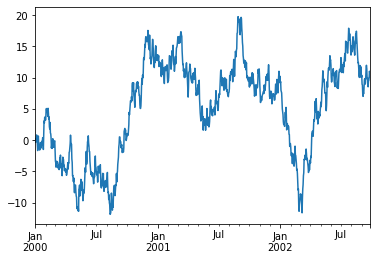
ts = pd.Series(np.random.randn(1000), index=pd.date_range('1/1/2000', periods=1000))
ts.head()
2000-01-01    0.127825
2000-01-02   -0.463126
2000-01-03    0.292114
2000-01-04    0.646686
2000-01-05    0.225687
Freq: D, dtype: float64
ts = ts.cumsum() #累加
在Pandas中可以使用.plot()直接绘图,支持多种图形和自定义选项点击可以查阅官方文档
ts.plot()
<AxesSubplot:>
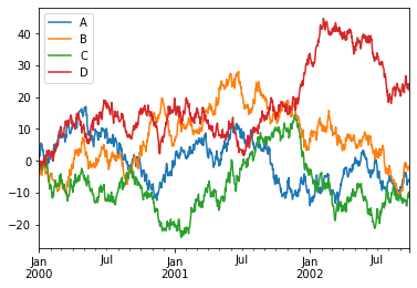
df = pd.DataFrame(np.random.randn(1000, 4), index=ts.index,
                  columns=['A', 'B', 'C', 'D'])
df = df.cumsum()
使用plt绘图,具体参数设置可以查阅matplotlib官方文档
plt.figure(); df.plot(); plt.legend(loc='best')
<matplotlib.legend.Legend at 0x7fc5990c00a0>
<Figure size 432x288 with 0 Axes>
导入导出数据
将数据写入csv,如果有中文需要注意编码
# df.to_csv('foo.csv')
从csv中读取数据
# pd.read_csv('foo.csv').head()
将数据导出为hdf格式
# df.to_hdf('foo.h5','df')
从hdf文件中读取数据前五行
# pd.read_hdf('foo.h5','df').head()
将数据保存为xlsx格式
# df.to_excel('foo.xlsx', sheet_name='Sheet1')
从xlsx格式中按照指定要求读取sheet1中数据
# pd.read_excel('foo.xlsx', 'Sheet1', index_col=None, na_values=['NA']).head()